Gradient Descent Implementation

We implement batch gradient descent from scratch and use it to minimize two toy objectives, following the treatment in Dive into Deep Learning, Chapter 12.3 [Zhang et al., 2021] — rewritten here to depend only on NumPy, PyTorch and Matplotlib.

from abc import ABC, abstractmethod
from collections.abc import Callable

import matplotlib.pyplot as plt
import numpy as np
import torch

Optimizer Base Class

An optimizer owns the objective \(f\), its gradient \(\nabla f\), and a learning rate \(\eta\). Concrete optimizers implement step, which maps the current weights to the next iterate.

class Optimizer(ABC):
    """Base class for iterative first-order optimizers."""

    def __init__(
        self,
        f: Callable[[float | np.ndarray], float | np.ndarray],
        grad_f: Callable[[float | np.ndarray], float | np.ndarray],
        lr: float,
    ) -> None:
        self.f = f
        self.grad_f = grad_f
        self.lr = lr

    @abstractmethod
    def step(self, weights: float | np.ndarray) -> float | np.ndarray:
        """Advance one iteration from ``weights`` and return the next iterate."""

Gradient Descent

Batch gradient descent implements the update rule

\[ \mathbf{w}^{(t+1)} = \mathbf{w}^{(t)} - \eta \nabla f\left(\mathbf{w}^{(t)}\right) \]

and records every iterate so that we can visualize the optimization trajectory.

class GradientDescent(Optimizer):
    """Batch gradient descent with a constant learning rate."""

    def __init__(
        self,
        f: Callable[[float | np.ndarray], float | np.ndarray],
        grad_f: Callable[[float | np.ndarray], float | np.ndarray],
        lr: float,
    ) -> None:
        super().__init__(f, grad_f, lr)
        self.weights_history: list[float | np.ndarray] = []

    def step(self, weights: float | np.ndarray) -> float | np.ndarray:
        if not self.weights_history:
            self.weights_history.append(weights)
        new_weights = weights - self.lr * self.grad_f(weights)
        self.weights_history.append(new_weights)
        return new_weights

One-Dimensional Example

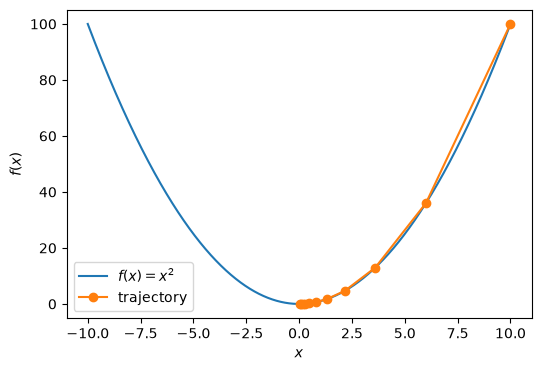
Minimize \(f(w) = w^2\), whose gradient is \(f'(w) = 2w\). Starting from \(w^{(0)} = 10\) with \(\eta = 0.2\), each update is \(w^{(t+1)} = w^{(t)} - 0.4 w^{(t)} = 0.6 w^{(t)}\), so the iterates contract toward the minimizer \(w^\star = 0\) by a factor of \(0.6\) per step.

def f(w: float) -> float:
    """Objective f(w) = w^2."""
    return w**2


def grad_f(w: float) -> float:
    """Gradient f'(w) = 2w."""
    return 2 * w


batch_gd = GradientDescent(f=f, grad_f=grad_f, lr=0.2)

weights = 10.0
for _ in range(10):
    weights = batch_gd.step(weights)

print([round(w, 4) for w in batch_gd.weights_history])

[10.0, 6.0, 3.6, 2.16, 1.296, 0.7776, 0.4666, 0.2799, 0.168, 0.1008, 0.0605]

def show_trace(f: Callable[[np.ndarray], np.ndarray], results: list[float]) -> None:
    """Plot f and the optimization trajectory over it."""
    bound = max(abs(min(results)), abs(max(results)))
    line = np.arange(-bound, bound, 0.01)
    _, ax = plt.subplots(figsize=(6, 4))
    ax.plot(line, f(line), label="$f(x) = x^2$")
    ax.plot(results, [f(x) for x in results], "-o", color="#ff7f0e", label="trajectory")
    ax.set_xlabel("$x$")
    ax.set_ylabel("$f(x)$")
    ax.legend()
    plt.show()


show_trace(f, batch_gd.weights_history)

Two-Dimensional Example

Next, minimize

\[\begin{split} f(\mathbf{w}) = w_1^2 + 2 w_2^2, \qquad \nabla f(\mathbf{w}) = \begin{bmatrix} 2 w_1 \\ 4 w_2 \end{bmatrix} \end{split}\]

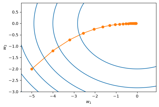
starting from \(\mathbf{w}^{(0)} = (-5, -2)\) with \(\eta = 0.1\). The two coordinates decay at different rates because the curvature along \(w_2\) is twice that along \(w_1\).

def f_2d(w: np.ndarray) -> np.ndarray:
    """Objective f(w) = w1^2 + 2 * w2^2."""
    return w[0] ** 2 + 2 * w[1] ** 2


def grad_f_2d(w: np.ndarray) -> np.ndarray:
    """Gradient [2 * w1, 4 * w2]."""
    return np.asarray([2 * w[0], 4 * w[1]])


batch_gd_2d = GradientDescent(f=f_2d, grad_f=grad_f_2d, lr=0.1)

weights_2d = np.asarray([-5.0, -2.0])
for _ in range(20):
    weights_2d = batch_gd_2d.step(weights_2d)

weights_2d

array([-5.76460752e-02, -7.31231688e-05])

Verifying the Gradient with Automatic Differentiation

The original notebook used the autograd package to differentiate the objective; the modern equivalent is torch.func.grad, which differentiates a function written with PyTorch operations. We use it to confirm our hand-derived gradient.

grad_f_2d_autodiff = torch.func.grad(lambda w: w[0] ** 2 + 2 * w[1] ** 2)

point = torch.tensor([-5.0, -2.0])
manual = grad_f_2d(point.numpy())
automatic = grad_f_2d_autodiff(point).numpy()
print(f"manual:    {manual}")
print(f"automatic: {automatic}")
assert np.allclose(manual, automatic)

manual:    [-10.  -8.]
automatic: [-10.  -8.]

def show_trace_2d(f: Callable[[np.ndarray], np.ndarray], results: list[np.ndarray]) -> None:
    """Plot the level sets of f and the optimization trajectory."""
    trajectory = np.stack(results)
    _, ax = plt.subplots(figsize=(6, 4))
    ax.plot(trajectory[:, 0], trajectory[:, 1], "-o", color="#ff7f0e")
    x1, x2 = np.meshgrid(
        np.arange(-5.5, 1.0, 0.1), np.arange(-3.0, 1.0, 0.1), indexing="ij"
    )
    ax.contour(x1, x2, f(np.stack([x1, x2])), colors="#1f77b4")
    ax.set_xlabel("$w_1$")
    ax.set_ylabel("$w_2$")
    plt.show()


show_trace_2d(f_2d, batch_gd_2d.weights_history)