Implement Queue using Stacks#
Problem#
Implement a First-In-First-Out (FIFO) queue using only two stacks. The
implemented queue should support all the functions of a normal queue, which are:
push, peek, pop, and empty.
The class MyQueue should include the following methods:
push(int x): Pushes elementxto the back of the queue.pop(): Removes the element from the front of the queue and returns it.peek(): Returns the element at the front of the queue.empty(): ReturnsTrueif the queue is empty,Falseotherwise.
Intuition#
Our main challenge here is that stacks are Last-In-First-Out (LIFO) structures, but we need to implement a First-In-First-Out (FIFO) structure using them. We can solve this problem by using two stacks, where one stack serves as a reversing mechanism.
When we push elements into the queue, we push them into the first stack. To pop an element, we need to get it from the bottom of the first stack. However, because we can only remove elements from the top in a stack, we transfer all elements from the first stack to the second stack, which reverses the order of the elements. Then, we can simply pop the top element from the second stack.
One easy way out which also works is just use one stack and use insert to push
elements to the bottom of the stack. However, this is not a good solution
because insert is an expensive operation. It takes \(O(n)\) time to insert an
element to the bottom of a stack of size \(n\).
Assumptions#
You must only utilize the standard operations of a stack: pushing to the top, peeking/popping from the top, checking its size, and checking if it’s empty.
Depending on your programming language, stacks might not be supported natively. However, you can simulate a stack using a list or a deque (double-ended queue) as long as you stick to the stack’s standard operations.
In our examples, we’ll be using Python’s
listto represent a stack. We will be using two stacks:The
enqueuestack: This stack is used for thepushoperation. In this stack, an element that is pushed first will be on the bottom and the element pushed last will be on the top. For instance, if we push 1, 2, 3, and 4 in this order, ourenqueuestack will look like[1, 2, 3, 4]. Here,1is at the front of the queue (the bottom of the stack) and4is at the back of the queue (the top of the stack).The
dequeuestack: This stack is used for thepopandpeekoperations. The order of the elements in this stack is the reverse of their order in theenqueuestack. If ourenqueuestack is[1, 2, 3, 4], ourdequeuestack will be[4, 3, 2, 1]. In this case,1is still at the front of the queue (now the top of the stack) and4is at the back of the queue (now the bottom of the stack).
Constraints#
The value that can be pushed into the queue (
x) is constrained by the range:\[ 1 \leq x \leq 9. \]The total number of function calls made to
push,pop,peek, andemptywill not exceed 100.All calls to
popandpeekfunctions will be valid.
What are Constraints for?#
In programming problems, constraints are set to define the scope and limits of the problem. They help us determine the feasible approaches and solutions for the problem by providing information about the range and characteristics of the input data. They also allow us to anticipate the worst-case scenarios that our algorithm should be able to handle without leading to inefficiencies or failures, such as exceeding the time limit or the memory limit.
In the context of the current problem:
The constraint on
x(i.e., \(1 \leq x \leq 9\)) specifies the minimum and maximum value that can be pushed into the queue. Knowing this, we can evaluate whether our solution would handle all possible values ofx. This constraint is important to consider when dealing with edge cases.The constraint on the number of function calls (i.e., at most 100 calls will be made to
push,pop,peek, andempty) informs us about the maximum operations our solution should handle efficiently. A solution with a time complexity of \(\mathcal{O}(n)\), where \(n\) is the number of operations, would likely be acceptable.The stipulation that all calls to
popandpeekfunctions will be valid simplifies the problem by indicating that we do not need to consider scenarios where these functions are called on an empty queue. This eliminates the need for additional error checking in our implementation.
Test Cases#
Test Case 1:
Operations:
push(5),push(6),push(7),pop(),push(8),peek(),pop(),pop(),push(9),empty()Queue states:
[],[5],[5,6],[5,6,7],[6,7],[6,7,8],[6,7,8],[7,8],[8],[8,9],[8,9]Expected Output:
None,None,None,5,None,6,6,7,None,FalseExplanation: After each push and pop operation, the queue state is updated. The peek operation does not change the queue state. The empty operation returns
Falsesince the queue is not empty.
Test Case 2:
Operations:
push(2),push(4),pop(),push(6),pop(),pop(),empty()Queue states:
[],[2],[2,4],[4],[4,6],[6],[],[]Expected Output:
None,None,2,None,4,6,TrueExplanation: After each push and pop operation, the queue state is updated. The empty operation returns
Trueas the queue is empty.
Edge Cases#
Edge Case 1:
Operations:
push(1),pop(),pop()Queue states:
[],[1],[],[]Expected Output:
None,1, Error messageExplanation: After pushing 1 and popping it, the queue is empty. Then the
pop()operation tries to remove an element from the empty queue. This should ideally throw an error or return a specific value indicating that the operation is not valid.
Edge Case 2:
Operations:
push(1),push(2),push(3),push(4),push(5),pop(),pop(),pop(),pop(),pop(),empty()Queue states:
[],[1],[1,2],[1,2,3],[1,2,3,4],[1,2,3,4,5],[2,3,4,5],[3,4,5],[4,5],[5],[],[]Expected Output:
None,None,None,None,None,1,2,3,4,5,TrueExplanation: This case tests the FIFO behavior of the queue after a sequence
Solution (Using Two Stacks)#
A queue operates on the principle of First In First Out (FIFO), meaning that the elements that are inserted first are the ones that get removed first. Commonly, queues are implemented using linked lists, with new elements being added to the rear and removed from the front. However, in this instance, we are implementing a queue using two stacks, which inherently operate on a Last In First Out (LIFO) basis. Here, elements are added and removed from the same end, known as the top.
To emulate the FIFO behavior of a queue using stacks, we need two of them. These two stacks collaboratively work to reverse the order of element arrival, effectively transforming the LIFO behavior of a stack into the FIFO behavior of a queue. Consequently, one of the stacks ends up holding the queue elements in the order they should logically be in if we were using a traditional queue structure. This innovative use of two stacks provides an alternative approach to implementing a queue data structure.
Implementation using List#
A small test suite is provided below to check the correctness of the algorithm.
Consider the case where we push 1,2,3,4 and then pop the first in queue and
then push 5, 6 to queue again and then pop the next in queue.
Our implementation still work in that case. Here’s the step-by-step breakdown:
You push 1, 2, 3, 4 to the queue. Now,
self.enqueue = [1, 2, 3, 4]andself.dequeue = [].You execute
pop(). Becauseself.dequeueis empty, you pop each element fromself.enqueuetoself.dequeue, resulting inself.enqueue = []andself.dequeue = [4, 3, 2, 1]. Then you pop fromself.dequeue, so you get 1, andself.dequeue = [4, 3, 2].Now, you push 5 and 6 to the queue. So,
self.enqueue = [5, 6]andself.dequeue = [4, 3, 2].If you execute
pop()again, it will pop fromself.dequeuesince it’s not empty, and you get 2. After the operation,self.enqueue = [5, 6]andself.dequeue = [4, 3].If you keep popping until
self.dequeueis empty, and then executepop()again, it will transfer elements fromself.enqueuetoself.dequeuejust like before.
1
2
Implementation using Stack Class#
1
2
Push#
The newly arrived element is always added on top of stack enqueue, see
Fig. 59.
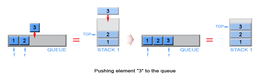
Fig. 59 Pushing an element onto the queue enqueue stack.#
Code Breakdown#
This push method is a part of the MyQueue class, which implements a queue
using two stacks: enqueue and dequeue.
Let’s break down what this push function is doing:
def push(self, x: int) -> None:
    """
    Pushes an integer x to the back of the queue.

    Parameters
    ----------
    x : int
        The integer to be added to the back of the queue.
    """
    self.enqueue.append(x)
The push method appends an integer x to the enqueue stack, which is used
as the main storage for incoming elements.
This mimics the behavior of a queue’s enqueue operation, adding an element to
the back of the queue. In a typical queue implementation, new elements are
always added to the end (or back) of the queue. Here, we simulate this by
pushing new elements onto the enqueue stack.
Time Complexity#
The time complexity of the push operation in this queue implementation is
\(\mathcal{O}(1)\). This is because the push operation essentially involves an
append operation to the end of the enqueue list, which is a constant time
operation in Python.
To understand this in a more practical sense, consider the following line from
the push method:
self.enqueue.append(x)
This line performs an append operation on the enqueue list. In Python,
appending to the end of a list is a constant time operation, meaning it takes a
constant amount of time to execute, regardless of the size of the list.
Therefore, the time complexity of the push operation is \(\mathcal{O}(1)\).
Case |
Complexity |
|---|---|
Worst Case |
\(\mathcal{O}(1)\) |
Average Case |
\(\mathcal{O}(1)\) |
Best Case |
\(\mathcal{O}(1)\) |
Space Complexity#
Type |
Complexity |
Description |
|---|---|---|
Auxiliary Space |
\(\mathcal{O}(n)\) |
The |
Total Space |
\(\mathcal{O}(n)\) |
The total space is the sum of the input and auxiliary space. Since the input space is \(\mathcal{O}(1)\) (no data given at the start), the total space complexity remains \(\mathcal{O}(n)\). |
Note carefully we treated both the enqueue and dequeue stacks as auxiliary
space. This is because they are not part of the input, but rather are used to
help in the operations of the queue.
Pop#
When the queue needs to be popped, we flip the enqueue stack and pour it into
the dequeue stack, see {numref}232_queue_using_stacksAPop for a visual
representation.
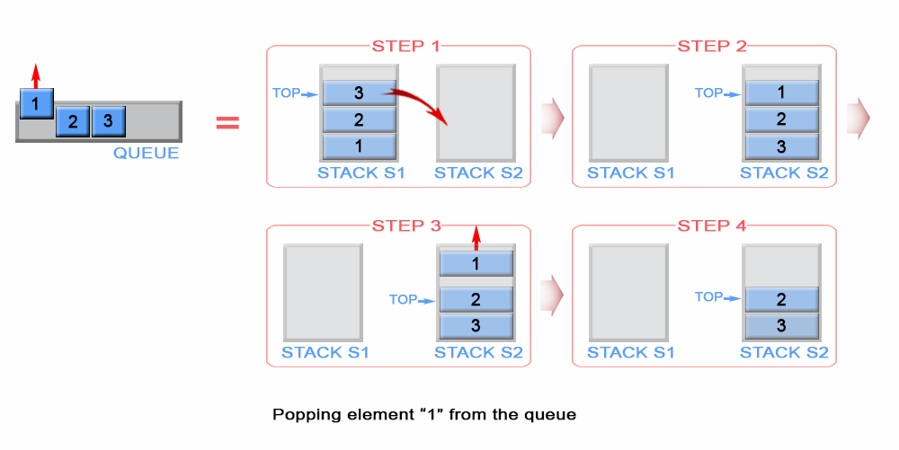
Fig. 60 Popping an element from the queue dequeue stack.#
Code Breakdown#
This pop method is a part of the MyQueue class, which implements a queue
using two stacks: enqueue and dequeue.
Let’s break down what this pop function is doing:
def pop(self) -> int:
    """
    Removes an integer from the front of the queue and returns it.

    Returns
    -------
    int
        The integer at the front of the queue.

    Raises
    ------
    IndexError
        If both stacks are empty, indicating the queue is empty.
    """
    if self.is_stack_empty(self.dequeue):
        self.move()
    return self.dequeue.pop()
The pop method simulates the behavior of a queue’s dequeue operation,
removing an element from the front of the queue. If the dequeue stack is
empty, it calls the move method to transfer all elements from the enqueue
stack to the dequeue stack, reversing their order to maintain the correct
queue order. It then pops and returns the top element from the dequeue stack,
which corresponds to the front of the queue.
Time Complexity#
The time complexity of the pop operation is not always constant because it
depends on whether the dequeue stack is empty. If the dequeue stack is not
empty, then popping an element off the dequeue stack is a constant time
operation, \(\mathcal{O}(1)\).
However, if the dequeue stack is empty, we need to transfer all elements from
the enqueue stack to the dequeue stack using move method, which takes
\(\mathcal{O}(n)\) time, where \(n\) is the number of elements in the enqueue
stack.
However, if we use
amortized analysis, we
see that for \(n\) push operations, there could be at most \(n\) pop operations
that transfer elements from enqueue to dequeue. Thus, in an amortized sense,
each pop operation takes constant time, giving us an amortized time complexity
of \(\mathcal{O}(1)\) for the pop operation.
Case |
Complexity |
|---|---|
Worst Case |
\(\mathcal{O}(n)\) |
Amortized Case |
\(\mathcal{O}(1)\) |
Best Case |
\(\mathcal{O}(1)\) |
Space Complexity#
The reason that the space complexity of the pop operation is considered
\(\mathcal{O}(1)\) is because the pop operation itself does not require any
additional space that scales with the size of the input.
When you call the pop method, it does not create any new data structures or
variables that depend on the size of the input (the number of elements in the
queue). Even when the pop operation triggers the move operation, no new
space is allocated; instead, the existing space in the enqueue and dequeue
stacks is reorganized.
The enqueue and dequeue stacks already exist as part of the queue’s storage,
so their space usage is considered part of the total space complexity of the
queue, not the auxiliary space complexity of the pop operation. The auxiliary
space complexity considers only the additional space required to perform the
operation, beyond the space already used to store the input.
So, while the total space complexity of the MyQueue class is \(\mathcal{O}(n)\),
where n is the number of elements in the queue, the space complexity of the
pop operation is \(\mathcal{O}(1)\) because it doesn’t require any additional
space beyond what’s already used to store the elements in the queue.
Type |
Complexity |
Description |
|---|---|---|
Auxiliary Space |
\(\mathcal{O}(1)\) |
See explanation above. |
Total Space |
\(\mathcal{O}(1)\) |
The total space is the sum of the input and auxiliary space. Since the input space is \(\mathcal{O}(1)\) (no data given at the start), the total space complexity remains \(\mathcal{O}(1)\). |
Armortized Analysis#
We will use s1 to represent the enqueue stack and s2 to represent the
dequeue stack for the following analysis.
I was genuinely confused by the amortized analysis of the pop operation when I
first encountered it. I didn’t understand how we could say that the amortized
time complexity of the pop operation was \(\mathcal{O}(1)\) when the worst-case
time complexity was \(\mathcal{O}(n)\) (seemingly).
Firstly, amortized time complexity is different from the worst-case time complexity. For the worst-case time complexity, we look at the scenario where the most unlucky thing can happen (i.e. finding the desired number only at the last element of a list). However, for the amortized time complexity, we average the time taken by all operations in a sequence, this sequence can be defined as the worst-case sequence of operations[1].
The basic idea is that a worst case operation can alter the state in such a way that the worst case cannot occur again for a long time, thus amortizing its cost.
The key to understanding why these queue operations have O(1) amortized time
complexity is understanding that each individual element is only moved once from
the enqueue stack to the dequeue stack.
Let’s consider a sequence of \(n\) push operations followed by \(n\) pop/peek
operations:
Each
pushoperation is clearly O(1). And so \(n\)pushoperations are \(\mathcal{O}(n)\).The worst case time complexity of a single pop operation is \(\mathcal{O}(n)\), since we have \(n\)
popoperations, the total time complexity is \(\mathcal{O}(n^2)\).
Remark 73 (Analyzing Time Complexity with Worst Case Only)
If we only consider the worst-case time complexity for the pop operation, it
could lead us to an overly pessimistic time complexity estimate.
Here’s a breakdown of the scenario:
We begin with an empty queue.
We push \(n\) elements into the queue. Each
pushoperation has a time complexity of \(\mathcal{O}(1)\), so \(n\)pushoperations have a time complexity of \(\mathcal{O}(n)\).We then pop all \(n\) elements from the queue. Each
popoperation could potentially have a worst-case time complexity of \(\mathcal{O}(n)\) when thes2stack is empty.
Now, if we were to look only at the worst-case time complexity of the pop
operation, we might think that popping \(n\) elements from the queue would have a
time complexity of \(\mathcal{O}(n^2)\), because for each pop operation we’re
considering its worst-case scenario, which is \(\mathcal{O}(n)\), and we’re doing
this \(n\) times.
However, this would be overly pessimistic as the bound given by the worst case
analysis is very “loose”. In reality, the worst-case scenario for a pop
operation (i.e., the s2 stack being empty and needing to move all elements
from s1 to s2) only happens once for every \(n\) push operations. After the
elements have been moved to s2, all the remaining pop operations have a time
complexity of \(\mathcal{O}(1)\) until s2 becomes empty again. In other words,
the number of times pop operation can be called is limited by the number
of push operations before it.
Therefore, the overall time complexity for \(n\) pop operations is not
\(\mathcal{O}(n^2)\), but closer to \(\mathcal{O}(n)\), leading to an amortized time
complexity of \(\mathcal{O}(1)\) per operation. Let’s proceed to prove it.
Example 51 (Amortized Time Complexity of Queue Operations)
Let’s break down the operations and their costs:
Each
pushoperation costs \(1\) unit of time, as it involves a singleappendoperation to the end of stacks1. Therefore, \(n\)pushoperations cost \(n\) units of time.The first
popoperation after a sequence of push operations is more expensive, as it involves popping all elements from stacks1and pushing them to stacks2. This costs \(2n\) units of time (one for eachpopfroms1, and one for eachpushtos2).However, once the elements are in stack
s2, each subsequentpopoperation only costs \(1\) unit of time, as it simply involves popping an element off the top ofs2. Therefore, \(n - 1\) such pop operations cost \(n - 1\) units of time.
So, the total cost of performing \(n\) push operations and \(n\) pop operations is
However, we performed \(2n\) operations in total (each push and each pop is
considered an operation), so the average cost per operation is
Note carefully the difference in units, the numerator is in time units, while the denominator is in number of operations. So the end result is in time units per operation, which coincides with the definition that on average, each operation takes \(2 - \frac{1}{2n}\) time units.
So when you compute \(\frac{(4n - 1)}{2n}\), you’re effectively asking: “On average, how many computational steps (time units) does each operation take?” This is the definition of amortized time complexity.
As \(n\) approaches infinity (which is usually the case when we talk about time complexity), the \(\frac{1}{2n}\) term becomes negligible, and so the amortized time complexity is approximately \(2\), which is a constant. Therefore, we say that the amortized time complexity is \(\mathcal{O}(1)\).
or more concisely,
The concept of amortized analysis is used in algorithms to show that while an operation might be expensive in the worst case, over time, the average cost per operation is much lower.
In this scenario, the expensive operation (pop operation when s2 is empty) does
not happen very often - it only happens when all elements need to be transferred
from s1 to s2, which happens once for every \(n\) operations. Thus, the cost
of this expensive operation is “amortized” over the \(n\) operations, resulting in
an average cost of \(\mathcal{O}(1)\) per operation.
Peek#
Same as pop, except we don’t remove the element from s2.
Empty#
Both s1 and s2 must be empty for the queue to be empty. The time and space
complexity of the empty operation are both trivial, \(\mathcal{O}(1)\).